BRFSS | Population-Level Prediction of Diabetes from Lifestyle and Behavioral Risk Factors
Background
Diabetes is the seventh leading cause of death in the United States, and a major public health problem around the world. The American Diabetes Association estimates the current national cost of diagnosed diabetes at ~$300bn per year, an amount that is likely to rise in coming years with increasing diabetes prevalence.
Data science efforts within health informatics have recently sought to discover risk factors for the disease beyond those already known (i.e., hypertension, cholesterol levels). For example, by studying large-scale medical claims data, a number of novel risk factors have recently been found for the disease, such as chronic liver disease and chronic bronchitis (Razavian et al., 2016). Yet, there remains plenty of scope for further exploration of possible risk factors, using more diverse datasets that relate to broader lifestyle factors (i.e., social, economic, or behavioral risk factors).
The Behavioral Risk Factor Surveillance System (BRFSS) is one such dataset: a survey administered annually in the US, with questions on the demographic background, health, and behavioral profile of respondents (e.g., healthy eating behaviors, exercise behaviors, etc.). Below, I develop a machine-learning approach to discovering potential risk factors for diabetes from this dataset. I ask the following question:
- Can the population-level prediction of diabetes be improved by including broad demographic, health, and behavior-related information in predictive models?
Exploratory Analysis
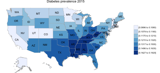
As a starting point in thinking about this question, I carried out a quick exploratory analysis of the BRFSS data, examining the prevalence of diabetes across the country. Historically, the percentage of the population with diabetes diagnosis was in the range of 5-10%; however, recent years have seen a sharp increase in this number, with prevalence of up to 10-15% in different segments of the US population. In addition, as illustrated in the panel below, there are clear asymmetries in the prevalence of diabetes by state, with a substantially higher proportion of the population in South Eastern states suffering from diabetes than in other regions of the US.
While I am not aware of any established linkage between, for example, healthy eating behaviors and diabetes prevalence, there are potentially broad demographic and lifestyle factors at play. For example, if healthy eating behaviors (i.e., fruit/vegetable consumption) varied systematically across regions of the country, this might play some role in disease prevalence at a population level.
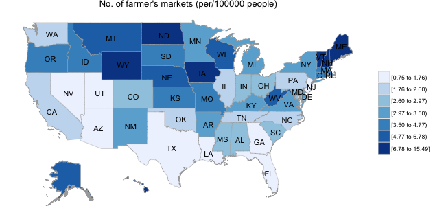
In the second panel below, I illustrate data obtained from the USDA website; specifically, I obtained the location of all farmer’s markets in the US, and calculated the number of markets per 100,000 population separately for each state. Interestingly, the distribution of farmer’s markets runs in stark contrast to the diabetes prevalence map, with as many as 6-10 times the number of farmer’s markets in Mid-Western states than in those states with high diabetic populations.
Below, I explore more systematically the role of lifestyle factors in diabetes prediction using the BRFSS data.
Data Preparation for Model-Fitting
In model-fitting, I focused on the period from 2011-2015, and specifically data from those odd years (2011, 2013, and 2015) that contained questions related to hypertension and cholesterol. Data for each year (SAS versions) were loaded into RStudio (Version 0.99) running on a local machine, and combined into one larger dataset. In total, the combined dataset contained approximately 1.5million respondent records. I decided to compare two predictor sets made up of 4 and 16 features respectively:
- Standard model: blood pressure, cholesterol, heart attack, stroke
- Extended model: standard model + 12 lifestyle/behavioral predictors (e.g., health rating, alcohol use, fruit/vegetable consumption)
In extracting, recoding, and transforming the variables of interest, I aimed for the clearest possible standardization, binarizing questions where possible, and dummy-encoding multi-leveled categorical questions. For example, for the healthy eating variables (e.g., units of fruit/vegetable consumed per day), a log transformation did not seem reasonable after initial exploration: even though these were rightward-tailed distributions, a very large no. of responses of “Never” were present (i.e., no consumption of fruit/vegetables). Thus, I chose to binarize these magnitude variables using a rule-of-thumb threshold, to create relatively balanced distributions (e.g., <0.33 units of fruit/day = Insufficient; >0.33 units of fruit/day = Sufficient).
In total, for the extended model there were 10 binary variables, 2 asymmetric binary variables (i.e., rare events like heart attack), and 4 categorical variables. A subset of the variable encodings are illustrated below:
> glimpse(brfssdata)
Observations: 1,439,696
Variables: 18
$ X_STATE  <dbl> 1, 1, 1, 1, 1, 1, 1, 1, 1, 1, 1,...
$ DIABETE3 <dbl> 0, 0, 0, 0, 0, 1, 0, 0, 0, 0, 0,...
$ BPHIGH4  <fctr> 1, 1, 1, 0, 1, 1, 1, 1, 0, 1, 0...
$ TOLDHI2  <fctr> 1, 0, 0, 0, 0, 1, 0, 1, 0, 0, 1...
$ CVDINFR4 <fctr> 0, 0, 0, 0, 0, 0, 0, 0, 0, 0, 0...
$ CVDSTRK3 <fctr> 0, 0, 0, 0, 0, 0, 0, 0, 0, 0, 0...
In passing, note that the asymmetric binary variables were left as is in the logistic regression, but that a clustering algorithm explored further below accounts for asymmetric binary variables in calculating distance. For all variables, Missing/’Don’t Know’ responses were not inputed, but simply coded as zero. Finally, for the dependent variable of interest (diabetes diagnosis), I chose not to include pre-diabetes or ’diabetes during pregnancy only’ respondents.
Logistic Regression: Standard and Extended Models
I built a logistic regression model for each of the two variable sets (Standard/Extended). The preprocessed data, which consisted of ~1,500,000 rows x 35 columns after dummy encoding, was first split into training (65%) and test (35%) sets. Each model was first fit to the training set, using a 10-fold cross-validation procedure and with L1 regularization as the feature selection approach. L1 regularization penalizes the model log-likelihood by adding to it the sum of the absolute values of variable coefficients; with an appropriately chosen penalty weight (lambda), this approach forces small beta weights towards zero, aiding in the exploration of the most predictive features in the data. I searched across a set of five lambda values.
Models were fit using R’s glmnet package, using code similar to below:
# split into training/test sets
split <- .65
randInd = runif(nrow(Xy))
train <- Xy[(randInd <= split), ]
test <- Xy[(randInd > split), ]

# prepare variables for logistic regression
k <- 10 #no. cross-validation folds
lseq <- c(.0001, .001, .01, .1, 1, 10) #regularization weights

# fit standard/extended models to training dataset using k-fold cv
smodel <- cv.glmnet(x = train[,1:5], y = train[,35], alpha = 1,
                         lambda = lseq, nfolds = k, family = 'binomial',
                         type.measure = 'auc')
emodel <- cv.glmnet(x = train[,1:34], y = train[,35], alpha = 1,
                         lambda = lseq, nfolds = k, family = 'binomial',
                         type.measure = 'auc')
Model Evaluation
To evaluate model performance, I compared the area under the ROC curve (AUC) for each model when applied to the test set, at a fixed lambda value of 0.001 (given time constraints, I did not attempt to bootstrap the estimated AUC values to provide a p-value). Interestingly, the additional demographic, health, and behavioral variables appear to improve the overall predictive power of the model relative to the standard predictors, with the extended model (16 variables) having an AUC of 0.81 compared to an AUC of 0.76 for the standard model (4 variables). This improvement is probably not surprising given the coarseness of the standard model, and the number of additional predictors added in the extended model; nevertheless, inspection of the model coefficients might tell us whether specific behaviors such as healthy eating play a role in improving prediction.
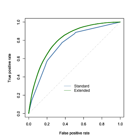
On inspection of the coefficients, however, NONE of the healthy eating behaviors appeared to be predictive of diabetes diagnosis (absolute value of all beta coefficients < 0.15).
Instead, the improved model performance appeared to be carried by the response trends in a categorical general health question: self-ratings of health on a 5-point scale from “Excellent” (beta weight = -1.39) to “Poor” (beta weight = 0.69) (for reference, the weights for blood pressure and cholesterol predictors were 1.1 and 0.73 respectively). Interestingly, the predictor for alcohol usage in the past 30 days showed a moderately-sized negative weight (-0.57), perhaps reflecting a tendency amongst people diagnosed with diabetes to avoid alcohol consumption.
In sum, the extended model improved on the prediction of diabetes diagnosis; however, there was no clear indication that this arose from the inclusion of factors as specific as healthy eating behaviors per se.
Cluster Analysis
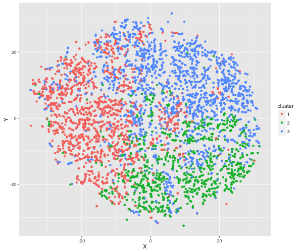
In a brief final exploration of the data, I developed a clustering algorithm that handles the mixed data types found in the BRFSS (thanks to a former Insight Fellow D. Martin for first illustrating for me the use of this method). Specifically, for a subset of 5,000 respondents with diabetes, I calculated all possible distances between them using Gower distance. I then clustered the respondents into groups (using the ‘partitioning around medoids’ method, k = 3 clusters), and examined the resulting clusterings by eye.
Printed in the panel below are the breakdown of the clusters based on respondents’ answers to the general health and exercise questions. The clusters appear to be broadly distinguishable based on these variables e.g., Cluster 1 consists of primarily non-regular exercisers with very low health ratings. Below, I also illustrate the distribution of individuals within each cluster, using a dimension reduction technique called t-distributed Stochastic Neighbourhood Embedding (t-SNE).
[[1]]                 [[2]]                [[3]]
GENHLTH   EXERANY2    GENHLTH   EXERANY2   GENHLTH   EXERANY2
0:  9     0:1291      0:  5     0:219      0: 10     0: 658
1: 36     1: 416      1: 58     1:989      1: 59     1:1427
2:177                 2:270                2:329
3:323                 3:563                3:916
4:794                 4:206                4:471
5:368                 5:106                5:300
Conclusions
I built on prior attempts to discover novel risk factors for diabetes, by extending the search for novel risk factors to the BRFSS dataset. By comparing the performance of a standard model, which included known diabetes predictors such as blood pressure and cholesterol, to performance of a model that included broad lifestyle and behavioral factors, I conclude that lifestyle factors alone (e.g., healthy eating behaviors, exercise) DO NOT provide much improvement on diabetes prediction relative to the standard model.
While some improvement was seen with the extended model, this was likely driven by responses related to general health in particular. The question remains open as to whether a more detailed treatment of lifestyle and behavioral factors, and their possible interactions, could improve diabetes prediction.
